Sea-Thru-Impl
28 Jul 2022Implementation is open sourced at https://github.com/Teragion/Sea-Thru-Impl
Sea-Thru is an algorithm that removes the veiling effects of water in images taken underwater. It is presented by Derya Akkaynak and Tali Treibitz at CVPR 20191.
Open Access: Sea-Thru: A Method for Removing Water From Underwater Images
Bibliographic Info: 10.1109/CVPR.2019.00178
It takes the original image and a depth map of the same size for inputs, and output the recovered image.
MiDaS (by Intel Intelligent Systems Lab) is a project for predicting depth map from an arbitrary image2. In this implementation, we explore the possibility of using monocular depth interpreting techniques to facilitate the recovery by Sea-thru.
The authors did not provide any code accompanying the original paper, hence all of the implementation is done by myself. The images and depth maps are provided by the authors (see Data/Data.md).
Summary / Abstract
This paper is a recent advancement of technologies reconstructing image from underwater captures as if they were taken on the ground (by “removing the water”). The major contribution of this paper is:
- Pointed out that coefficients related to wideband attenuation $\beta^D$ and backscatter $\beta^B$ are different.
- Proposed a practical way of independently estimating these parameters with experiment-based interpolating techniques.
- Shown that both $\beta^D$ and $\beta^B$ are dominanted by their $z$ dependency.
Traditionally, $\beta^D$ and $\beta^B$ are considered as equivalent parameters. This results in significant distortion in some situations.
Sea-thru greatly improved the results of recovering the image from underwater captures, for detailed comparison of results, please refer to the original paper (as I have not implemented the traditional methods to compare).
Imaging Underwater
Water’s effects on an image taken underwater can be divided into two categories: wideband attenuation and backscatter. Specifically, underwater image $I$ is represented as
\[I_c = D_c + B_c\]where $c\in {r,g,b}$ representing each color channel. $D_c$ is the direct signal containing information of the attenuated scene, and $B_c$ is the backscatter due to water. They can be further decomposed as
\[\begin{aligned} D_c &= J_ce^{-\beta_c^D(\textbf{v}_D)z} \\ B_c &= B_c^\infty(1-e^{-\beta_c^B(\textbf{v}_B)z}) \end{aligned}\]where $\textbf{v}_D = {z, \rho, E, S_c, \beta}$ and $\textbf{v}_B = {E, S_c, b, \beta}$ representing $\beta_c^D$ and $\beta_c^B$ depend on range (depth) $z$, reflectance $\rho$, spectrum of ambient light $E$, spectral response of the camera $S_c$, and the physical scattering and beam attenuation coefficients of the water body, $b$ and $\beta$. There exist some direct fomulae to describe their relationships, but they are beyond the scope of this study.
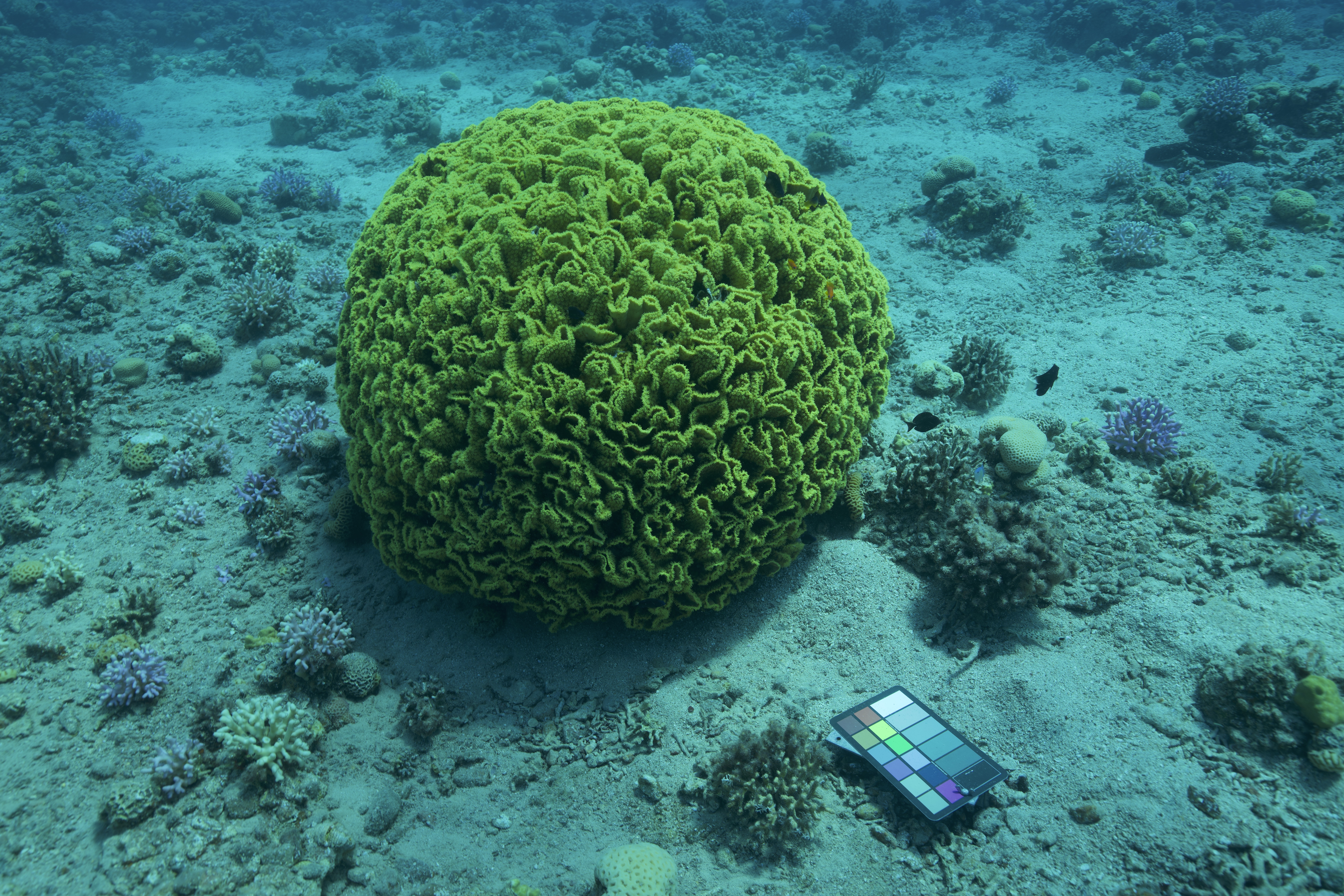
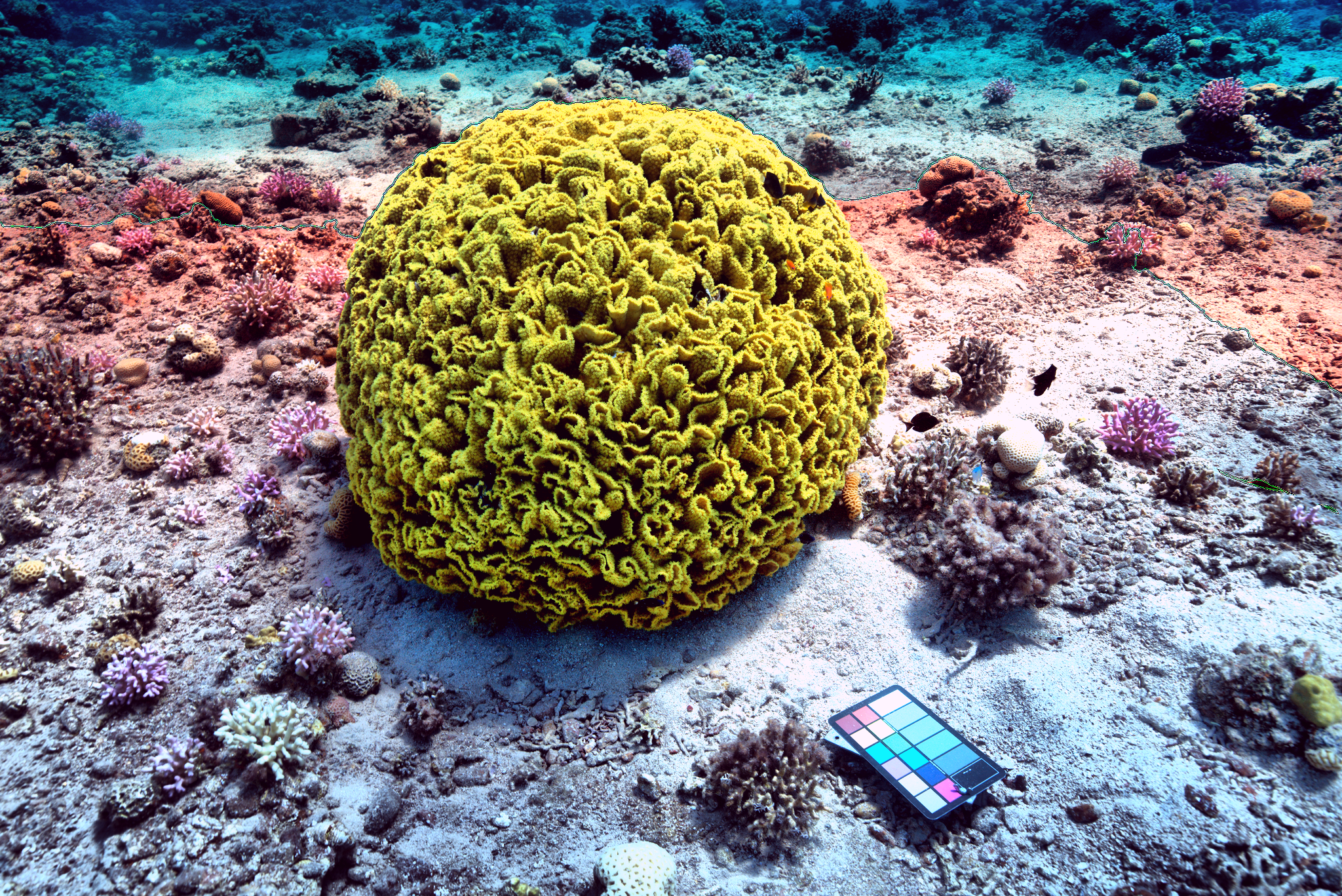
Example of image under water
It is, of course, desirable if we have all those parameters in mind, but this is generally not possible in practice. Hence, we make a strong assumption that is good enough visually that $\beta_c^D$ is almost dominant by $z$ and $\beta_c^B$ most strongly affected by $E$ (property of the environment).
Removing Backscatter

Relationship between image captured, direct signa and backscatter
The first step of image reconstruction is removing the $B_c$ for each color channel. This should be easy as $B_c$ does not at all depend on the color of the original image ($J_c$), but only the depth and the invariant water background.
The backscatter is estimated using
\[\begin{align*} \hat{B_c}(\Omega) &\approx I_c(\Omega) \\ \hat{B_c} &= B_c^\infty(1-e^{-\beta_c^Bz}) + J_c'e^{-\beta_c^{D\prime}z} \end{align*}\]$J_c’$ and $\beta_c’$ are constant parameters replacing the real value in the original formula. $\Omega$ is a set of points that is chosen from the original image by the following procedure:
- Divide all pixels into $k$ bins evenly spaced by their depths values (in practice we have $k=10$).
- From each bin, choose the points from the bottom $1\%$ of their
RGBnorm.
We then simply use scikit-learn’s curve_fit routine to find optimal parameters for $B_c^\infty$, $\beta_c^B$, $J_c’$, and $\beta_c^{D\prime}$. Using these parameters, we are able to compute $B_c$ for all pixels.
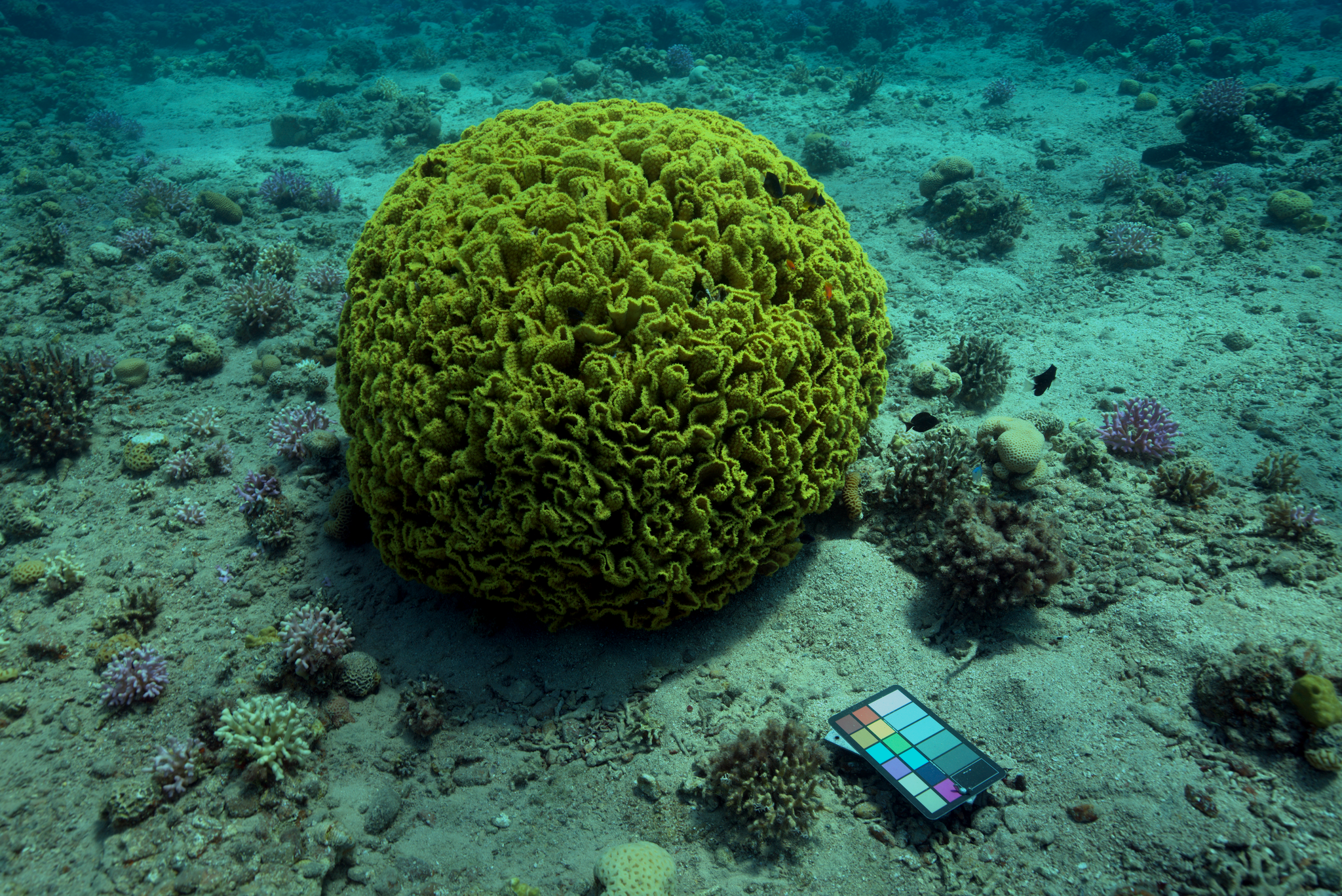
The original image with backscatter removed
Computing Wideband Attenuation
The next step would be estimating $J_c$ from $D_c$, which means to estimate $\beta^D(z)$. By the experiments of the authors of Sea-thru, it turns out that a 2-term exponential is good enough for interpolating $\beta_c^D$:
\[\beta_c^D(z) = a \cdot e^{b\cdot z} + c \cdot e^{d\cdot z}\]The experiment is mainly done by tracking the color chart boards placed in the scene and see how they were attenuated.
This is the major contribution of Sea-thru: instead of reusing the estimation for $\beta^B$ as $\beta^D$, the parameter for wideband attenuation is estimated in completely original way.
Preliminary Estimation
We use LSAC (Local Space Average Color) 3 method to compute an illuminant map $\hat{E_c}$ for the original image.
According to the original image, the colors should be computed as local averages of neighborhoods defined by
\[N_e(x,y) = \{(x',y')| \|z(x,y) - z(x',y')\|\leq \epsilon\}\]subject to the constraint that $(x’,y’)$ are four-connected.
However, to compute the neighborhoods in this way, it would require computation cost and storage space of $O(n^2)$ where $n$ is the resolution of the image. This is prohibitively expensive for practical situations.
Hence, instead of computing the neighborhood for each pixel, we segment the image to some neighborhoods such that each neighborhood extend in the four-connected way if the pixel next to it and the current pixel differ by less than $\epsilon$. This means that each pixel would only be in $1$ neighborhood, $O(n)$ complexity and storage. In practice, we see that this method performs good enough.

The illuminant map computed for the original image
After obtaining an estimation for $\hat{E_c}$, we compute a coarse estimation of $\beta_c^D$ by
\[\hat{\beta_c^D}(z) = -\log\hat{E_c}(z) / z\]Refine Estimation
This estimation is then refined using formula the same formula, but instead we optimize the parameters by predicting $z$.
That is, let
\[\hat{z} = -\log E_c/\beta_c^D(z)\]minimize
\[\|\hat{z} - z\|\]Again, this can be done using scikit-learn’s curve_fit routine.
In our case, this interpolation is the most costly operation in the pipeline. However, this is due to we naively use the depths at all points to interpolate. A better approach may be using some downsampled points without losing too much performance. If that is done, the entire algorithm is suited for real-time purposes.
Recovery
Finally, the original image is recovered as
\[I_c = J_c \cdot e^{\beta_c^Dz}\]Afterwards, we perform some calibrations for white balance (using the grey world assumption) and exposure.
Results and Discussion
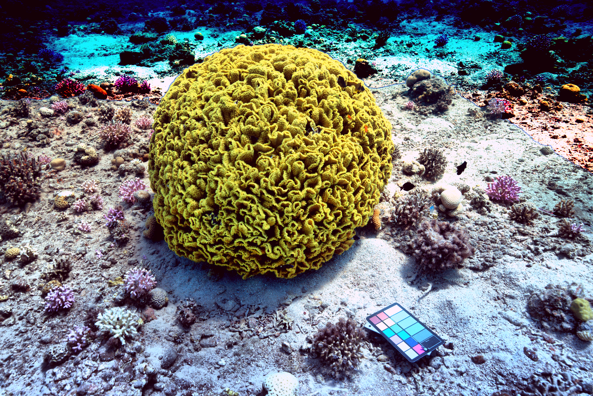
Recovered image using given depth map
This is the recovered image using Sea-thru for the example image and provided depth map. Note that although the major part is reconstructed perfectly, the top/right parts of the image is distorted and barely recognizable. This is because the depth information at this area is missing. Although it is possible to use information from other area to interpolate, it does not yield good results. Indeed, in the original publication, the result image simply have those regions without depth information cropped out.
Naturally, we think of using predicted depth map from MiDaS to substitute or facilitate interpolation, and here is the results:
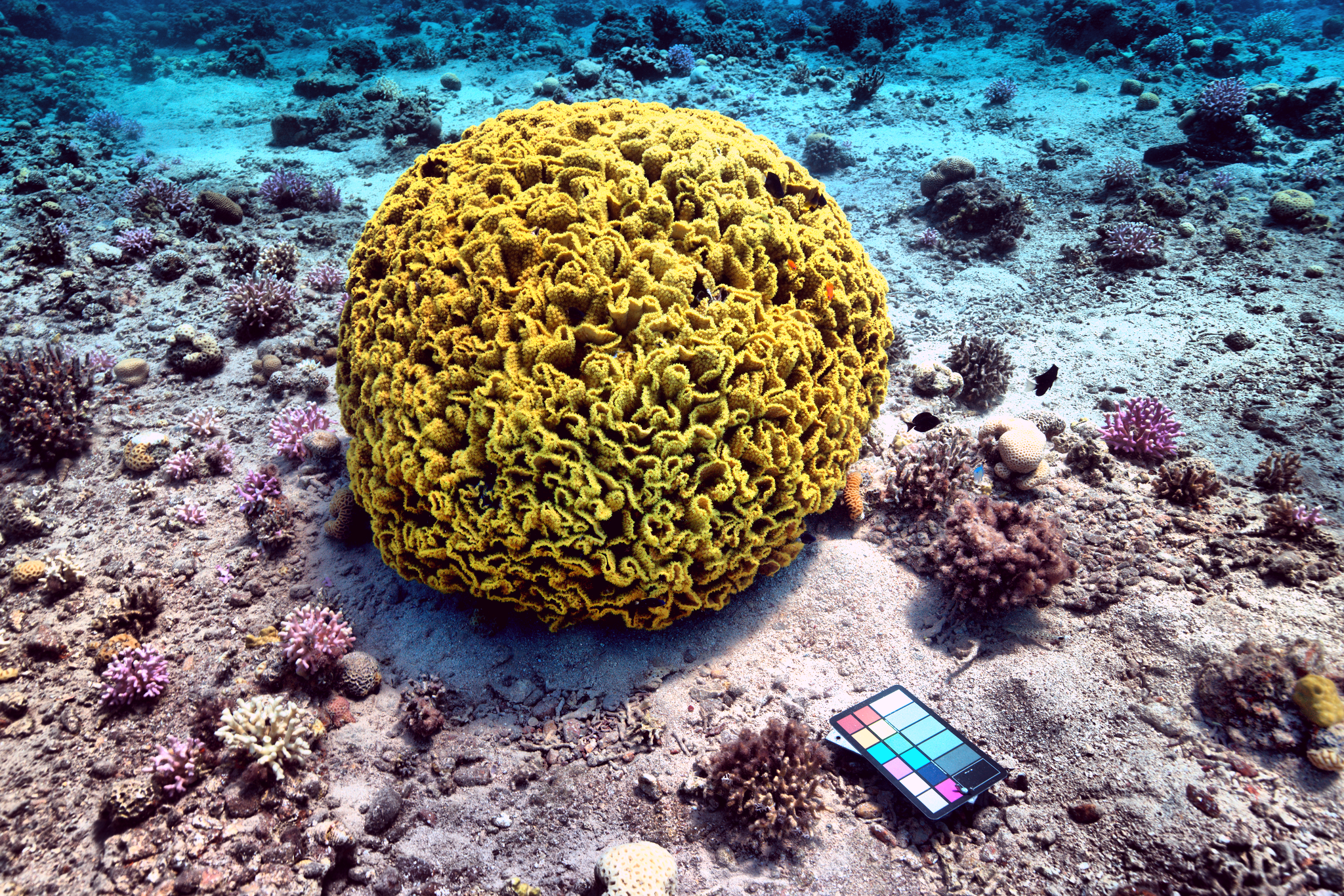
Recovered using predicted (top) depth map and interpolated (bottom)
There is still artifacts at the interpolated (probably due to my poor skill of stitching the depth maps together) and the predicted map has slightly worse color recovery. This could be due to the incompetency of MiDaS in reconstructing depth information under water. In fact, the predicted depths have significantly less contrast than the given depth map.
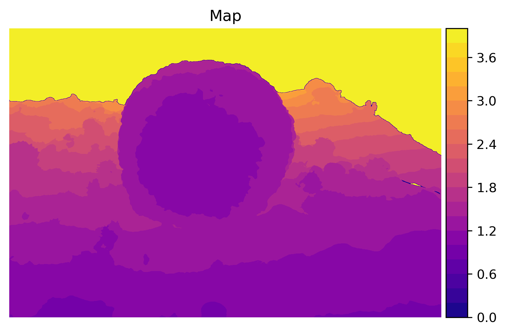
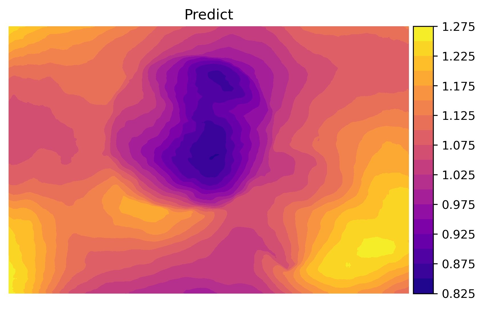
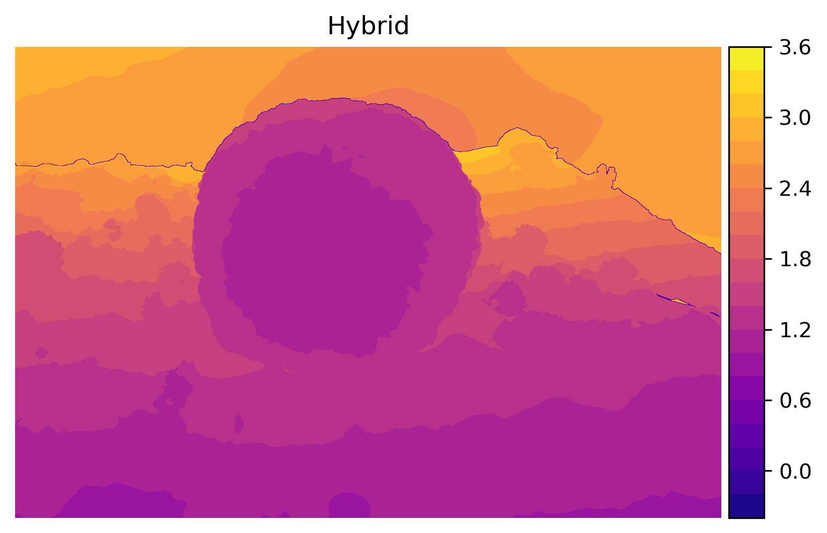
Comparison of depth maps of each method
This could be alleviated by retrain the model with underwater images, but unfortunately Intel ISL did not provide the access to the training code of MiDaS.
Nevertheless, all those methods provide acceptable results for image recovery, but obviously there is potential for improvements.
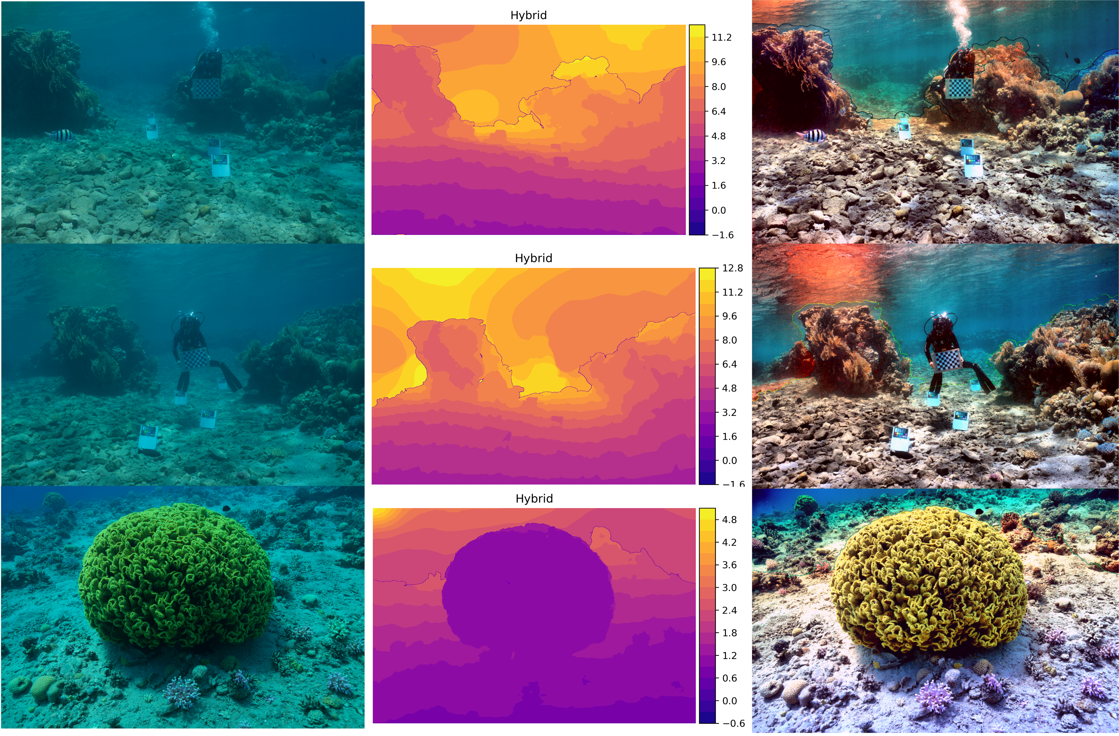
The recovery of some other images using hybrid method
Clearly, these methods perform well even with images where depth varies greatly. All those images somewhat suffer from a blue-ish attenuation at the far side, but again that is due to the missing of direct depth data and conservative estimation by MiDaS. Future study may be oriented in dealing with those areas.
Notes of implementation
This project is an implementation of the Sea-thru algorithm.
The implementations for the original paper are contained in files sea_thru.py, compute_illuminant.cpp, and simple_illuminant.cpp.
Folder midas/ contains a fork from repository isl-org/MiDaS which contains an implementation of paper Towards Robust Monocular Depth Estimation: Mixing Datasets for Zero-Shot Cross-Dataset Transfer from Intel ISL (please see LICENSE_MiDaS for permissions).
midas_helper.py is an interface written to call MiDaS from our implementation of Sea-thru.
Dependencies are those listed in sea_thru.py and midas_helper.py. Namely, the following python packages:
For Sea-thru:
numpyscikit-imagescikit-learnscipyopencvrawpy(to work on apple silicon Macs, you may need to installrawpyfrom source)
For MiDaS integration to work:
pytorchtorchvisiontimm
To compile C++ modules including compute_illuminant.cpp and simple_illuminant.cpp, use command like
/path/to/clang++ -O2 -o sillu.<OS specific suffix> -shared <src>.cpp -std=c++17 -lomp -fopenmp
where <OS specific suffix> is something like .so, .dylib, etc.
The code is implemented and tested under macOS.
Citations
-
D. Akkaynak and T. Treibitz, “Sea-Thru: A Method for Removing Water From Underwater Images,” 2019 IEEE/CVF Conference on Computer Vision and Pattern Recognition (CVPR), 2019. ↩
-
Ranftl, René, et al. “Towards Robust Monocular Depth Estimation: Mixing Datasets for Zero-Shot Cross-Dataset Transfer.” IEEE Transactions on Pattern Analysis and Machine Intelligence, 2020. ↩
-
M. Ebner and J. Hansen. Depth map color constancy. BioAlgorithms and Med-Systems, 9(4):167–177, 2013. ↩